FP6 AUTOMATION

Micro-Rotation Workbench

The Micro-Rotation Workbench (MRW) is part of the FP6 Automation Project.

• Note: In the project proposal it is named more accurately as Micro-Rotation Simulator (MRS).

The MRW simulates the rotation and movement of a 3D object, and the acquisition of 2D slices under certain microscopic conditions in a time series, thus producing a tomography of the object. (Not a projective standard tomography, but a real tomo - graphy, imaging slices!!!)

The original object is a 3D image that is rotated and shifted, then convolved to simulate an image acquisition with a Fluorescence Microscope (see Cookie Cutter) with some added Photon Noise.

The MRW can also provide a 3D Point Spread Function for the specified Microscopic Parameters instead of a rotation simulation. This is achieved by setting the "total time simulated" parameter to zero.

Location

The MRW is located at the Automation Project server as part of the Scientific Image Data Base (SIDB) there running. Login instructions to the MRW are sent to Automation partners privately.

Objects especially intended to be rotated in the simulator are grouped under a common image project. This can be directly accessed by clickin on the menu entry 'MRW'. The simulator (MRW) is one of the possible actions on each image of the list.

Conventions

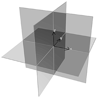
The optical axis goes along Z, and XY planes are captured at a fixed Z coordinate (the center of the original image) at equally distributed time points. The objective is supposed to be at lower Z coordinates, as in an inverted microscope.

The movement of the object is described with six parameters: three space coordinates for the center of the image, and three angles: rotation (R) precession (P) and nutation (N).



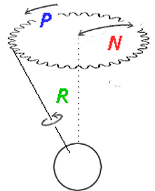
Concerning rotation: it is conceptually simulated in two steps. Think about it like this: the object is first rotated an angle R around a given main axis K (that you may select among X, Y and Z, but Z is not useful for tomography as it is the optical axis!!!). Afterwards it is tilted a given angle N around a precession vector L. The vector L is perpendicular to K, and rotates around it an angle P. This means that only two rotations (R, N) around two axes (K, L) occur, and four parameters are needed to describe them. These will be the angles R and N themselves, plus a parameter that describes the main axis of rotation K, plus a parameter P that describes how much is the precession vector L rotated around it.

Notice that this is not the standard definition of precession and nutation used for planets. We use the same terminology for the sake of simplicity, but the nutation here is the full angle that the axis of rotation is tilted from the main coordinate axis. The direction in which this tilt is done is determined by the precession angle.

A third rotation is possible at the begining of the simulation, to select what main axis of the object is oriented at first along the optical axis. After this first reorientation, whatever it is, the convention to describe the coordinate axes is like in the following illustration, with the origin at the center of the original image and the optical axis along Z.

Modelling pipeline

1. Rotate and translate rigid synthetic object at the 50 nm sampling grid using Trilinear Interpolation.
2. *More than 2× oversampled in the Widefield case, but less than that in the Nipkow case (this is restricted due to computing limitiations, but will work at 25 nm in the future).
3. (Extra step in the future, currently not necessary) downsample to 50 nm to speed up convolution in the next step.
4. Compute 3D convolution with the Point Spread Function for the appropriate optical conditions, including depth (to simulate Spherical Aberration)
5. Take out the 2D slice currently located at the center of the original image volume, which is the constant imaging coordinate.
6. Apply CCD cell model (convolution with a 2D square of the size of the cell), including downsampling by an integer factor.
7. Go to 1 until the full Time Series is calculated.
8. 'Add' Poisson noise.

You can obtain the Point Spread Function instead of a rotation simulation if you specify a zero value for "total time simulated". You can also skip the simulation and obtain only the table of coordinates by setting "coordinates table only" to one. See below.

Microscopic parameters

These are the parameters describing the optical conditions. Please refer to Microscopic Parameters for more details.

The original image has a particular Sampling Density, but the resulting image will be resampled multiplying this sampling by an integer factor to simulate the averaging behaviour of a CCD camera. You should not change the sampling density parameters of the original image, but the factor on the settings below.

Micro Rotation parameters

Preliminar settings

• Total time simulated: total time of simulation in arbitrary units. Most of the times you leave it in 1. If you make it 0, then no rotation is simulated, and the Point Spread Function is returned instead.
• Images per unit time: number of images acquired per unit time.
• Size of CCD cell: integer factor to multiply the original image Sampling Density to simulate the camera averaging behavior. Thus, if the original image had a sampling distance of 25 × 25 nm^2> in the XY plane, and this factor is 4, the sampling in the resulting image will be 100 × 100 nm².
• Signal to noise ratio: parameter describing the amount of Photon Noise in the resulting image. See Signal To Noise Ratio.
• Original axis oriented to Z. The original image, before the simulation begins, is rotated to place its axis here specified along the optical axis, to allow an extra degree of freedom. If this is set to "z", the original image is left as is, because it is already aligned with the optical axis Z.
• Initial depth and stepper speed for acquisition plane: these quantities, expressed in micrometers (µm) and in micrometers per unit time respectively, describe at what real depth inside the sample is the imaged plane, measured from the coverslip (which is located below the object, see conventions above). It is important in order to simulate the existance of Spherical Aberration, because it depends on the depth inside the sample. Spherical aberration arrises due to a Refractive Index mismatch, but it is negligible if the value of this parameter is zero (close to the coverslip). These parameters alter only the PSF for each imaged frame, not the position of the object. They must be combined with a linear movement of the object along the optical axis in order to make a realistic simulation of a micro-slicer, see center position below. When the stepper speed is zero, a constant PSF is used for all the time series.
• Coordinates table only: if this parameter equals 1 no simulation will run, and only the table of coordinates and rotations of the object along time will be returned. This can be useful to test different parameters before going to the more resource consuming simulation.

Center position

This is to describe the movement of the center of the object. The movement along each coordinate X, Y and Z is made of up to five components, which allow a lot of flexibility in the movement description. The components are: one Brownian Motion component, plus one constant value (actually, normally distributed with a mean value and a standard deviation σ), plus a shift caused by a constant speed, plus an oscillatory (cosine) component, plus a deterministic coordinate value from a data table. The total sum is given in terms of the size of the original image, where 1 is the total image size in a particular direction.

By having a constant speed component, and setting the oscillations and the rotations (see below) all to zero (or to fluctuating values to have some noise), we can simulate a micro-slicer too!!! The mean Z position (i.e. initial Z value) would then be 0.5 (the image moved upwards half of its height) and the Z constant velocity would be -1 (that will move the whole image downwards a full height in one time unit). Because the objective is supposed to be at lower Z coordinates, this simulates the acquisition of slices at deeper and deeper positions each time. We can combine this with a PSF depth-dependent variation as well to make a more realistic simulation!!! (See preliminar settings above).

Without any noise in the movement, this constant Z shift would be equivalent to a standard 3D stack measurement, but with the benefit of having all the imaged 2D planes at the same fixed depth inside the sample. In presence of Spherical Aberration that is actually very convenient, because it makes the Point Spread Function to be constant!!!

With the oscillatory component you can add all kind of perturbations to the constant speed: by adapting the frequency and the phase you can select the part of the cosine that will be added, from an almost linear slope to a curve that changes direction.


For every (x, y, z) component you have:

Brownian motion

• Brownian diffusion value: average total displacement per unit time. Brownian Motion is caused by random hits of the molecules in the surrounding medium.
• Brownian integration time: if = 0, this is a regular Brownian Motion that causes diffusion. If > 0, its value is used as a reduced time window in which the random hits are accumulated, effectively damping the movement.

Constant component

• Mean position: mean value of the normally distributed "constant" component.
• Sigma position: the standard deviation of that component.

Constant velocity

• Constant velocity: a constant speed for shift along this direction.

Oscillatory component

• Amplitude oscillation: peak-to-peak amplitude of the cosine oscillation. A value of one will make the center of the image swing from one side to the other of the original image, so half of the object is ouside the acquired image.
• Frequency oscillation: frequency in Hertz (complete oscillations per unit time).
• Phase oscillation: a starting phase for this component oscillation, in degrees (0 - 360).

Data table

Text files with ASCII data can be uploaded to the database and used as coordinates for the image position in the simulation. This allows the usage experimentally recorded data. If this is the only coordinates we want, we have to make the rest of the parameters = 0; otherwise it is considered just as an extra component that is added to the rest.

• File ID for coordinate table: the database ID (an integer number) that refers to a text file with columns of data, separated by spaces. No table is used it this value is left empty.
• Table column: index number that specifies which column of the table is used for this coordinate. The first column has index number 1.
• Coefficient for column: a real factor to multiply the value read from the table. Use a zero to have no table contribution to a given coordinate.

Given a column of the table, its first row is used for the coordinate of the first time frame in the series, its value multiplied by the coefficient. Then for each frame the next row is taken. If the end of the table is reached before the simulation ends, the index "bounces back", begining to decrease, reading the table backwards.

Some tables are already uploaded with ID ranging from 13 to 19, ready to use. These come from experimental data.

Rotation around main axis

You select a main axis of rotation (usually not the same as the optical axis) and describe the speed of rotation around it. The axis of rotation goes through the center of the original image. If you want the object to rotate with its axis away from the imaged plane, a shift can be added with the parameters for the center position (see above).

The rotation is described by its speed. The speed has a constant component (actually normally distributed, so you can specify a standard deviation to introduce some randomness) plus a time varying (cosine) component. This oscillating component will let you introduce acceletarions in the rotation of the object, depending on how you establish the parameters. For constant or approximately constant rotation speeds, leave its amplitude at zero.

• Rotation axis: this specifies along which axis of the original image the main rotation (R) occurs.
• Initial rotation angle: rotation angle at the begining of the simulation
• Mean rotation speed: speed of rotation, in turns per unit time.
• Sigma rotation speed: standard deviation of the mean rotation speed, as measured after a complete turn.
• Amplitude rotation speed: amplitude of the oscillating component of the rotational speed.
• Frequency rotation speed: frequency of the oscillating component, in Hertz (cicles per unit time)
• Phase rotation speed: initial phase of the oscillating component.

Precession and nutation

The precession and the nutation go together. The object, after rotation (R) with the above parameters, is tilted a given angle of nutation (N) around an axis specified by the precession vector (see conventions above).

As with the rotation, you describe the movement of the precession vector by its speed. If you want it fixed, the speed must be zero. If you do not want any tilting at all, the nutation value should be zero despite the actual value of the precession.

Again, the precession speed has a constant component plus an oscillating (cosine) component, that add up to give the total speed.

• Initial precession angle: the angle of the precession vector at the begining of the simulation
• Mean precession speed: mean value of the speed of rotation of the precession vector (in turns per unit time).
• Sigma precession speed: the standard deviation of the precession vector speed.
• Amplitude precession speed: amplitude of the oscillatory component of the precession speed, in turns per unit time.
• Frequency precession speed: the frequency of the oscillatory component.
• Phase precession speed: the phase of the oscillatory component at the begining of the simulation.

Nutation

Given the precession vector above, the object will be tilted a particular angle of nutation N.

This angle is now described by a constant (normally distributed) component plus an oscillatory component, similarly to previous cases. The two components add up to give the total angle of nutation.

• Mean nutation angle: in degrees (0 - 180)
• Sigma nutation angle: standard deviation of the mean angle in degrees.
• Amplitude nutation: in degrees (0 - 180)
• Frequency nutation: cicles per unit time of the angle oscillation.
• Phase nutation: phase of the oscillatory component at the beging of the simulation.

Output

After the simulation ends, the image is saved as a Time Series in ICSfile Format in a personal directory (-+tosidb+-) of the SIDB server. See To Sidb for more details.

Two links will appear allowing you to download the two parts of the image file: the ICS header (quite small) and the IDS data file (tipically much larger). The IDS file will be compressed (gzipped) for a faster download. You do not need to decompress it to open it with the Huygens Software, the program will do it on the fly.

Another link will let you download a text file containing a table with all the abovementioned coordinates describing the object movement along time.

All this files will remain in your To Sidb directory after you download them. You should delete them manually later after downloading, in order to keep the server unloaded.

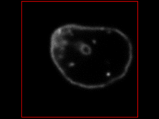
Some images

Take for example this object:

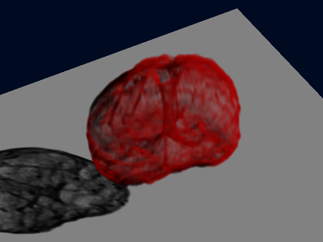<br /> Sfp Renderer

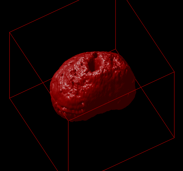<br /> Surface Renderer

Outputs from the simulator, under different conditions:

Smooth rotation with some movement<br />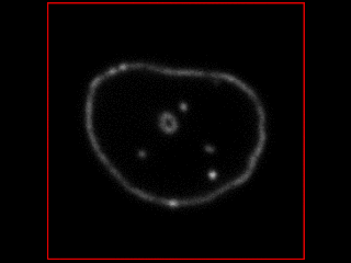


Crazy rotation with much shift <br />


Working as a slicer along Z <br />
<br />

Simulations for a Confocal Microscope