
Convolution
You can imagine that an image is formed in your microscope by replacing every original Sub Resolution light source by its 3D Point Spread Function (multiplied by the correspondent intensity). Looking only at one XZ slice of the 3D image, the result is formed like this:
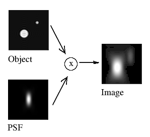 (Fig. 1)
This process is mathematically described by a convolution equation of the form
$$ g=h \ast f $$ (Eq. 1)
where the image g arises from the convolution of the real light sources f (the object) and the PSF h. The convolution operator * implies an integral all over the space:
$$ g=h \ast f = \int\limits_{-\infty}^{\infty}\int\limits_{-\infty}^{\infty}\int\limits_{-\infty}^{\infty} h(\vec x - \vec x') f(\vec x') d\vec x' $$ (Eq. 2)
Interpretation
Equation 2 can be interpreted as follows: the object "f" is split up in an infinite amount of tiny point-like fluorescing volumes. A point-like volume at $$ \vec x $$ emits $$ f(\vec x) $$ and makes a contribution to the image in the exact form of the Point Spread Function at a location in the image corresponding with $$ \vec x $$ in the object. Because of the incoherency of the fluorescence light, all contributions from all points add up to form the image.
In terms of voxels, each object voxel is substituted with a PSF with a strength proportional to the voxel's value and centered on its position. The sum of all these overlapping PSFs makes up the image.
Calculation
Convolving two functions is equivalent, in the Fourier domain, to multiply their Fourier Transforms. This speeds up the computations. See Cookie Cutter.
Reverting the procedure
DeConvolution (see) is the opposite mathematical operation, to recover an image that is degraded by the process of convolution.