
Ideal sampling for image acquisition
The ideal Sampling Density during image acquisition depends on the optics of the microscope. It is recommended to sample the image at a rate close to the ideal Nyquist Rate. Images obtained with sampling distances larger than those established by this rate are not well sampled.
Ideal means necessary to capture all the information. As the Point Spread Function (PSF) is the basic "brick" of which the images are "built", one should record details at least on the scale of the PSF to gather all the available information. Failing in that may spoil any attempt of doing deconvolution, because deconvolution works on the PSF scale. If your digital sampling occurs at a physical scale much larger than that of the PSF, deconvolution simply cannot happen!!! You would be recording many PSF's inside each image pixel, and it wouldn't be possible to disentangle them anymore. See Quality Vs Sampling.
Definition
Defining the ideal sampling in terms of Spatial Resolution is frequently done as a rule of thumb ("sample with half the Rayleigh Criterion"), but this is an ambiguous definition (there are many possible criteria for Spatial Resolution), and in some cases will lead to undersampling (see Pinhole and Bandwidth for example).
In terms of signal analysis the ideal sampling rate is better defined in terms of the system bandwidth, which is determined by the Point Spread Function. This is more precise because it considers the maximum frequency that the optical system can register, and it guarantees that all information is properly acquired. This ideal sampling is defined as the Nyquist rate. Most microscopes have a hard practical bandwidth limit, and this limit is dependent on the microscope type. The figure below shows the fluorescence intensity (in arbitrary units) as a function of the frequency (cycles/micron). STED microscopes do not have a bandwidth limit, i.o.w. it does not have a Nyquist rate. However, we can still define a 'practical' Nyquist rate for STED based on the attenuation of the bandwidth in the high frequency range. This attenuation is dependent on the STED depletion intensity, STED wavelength and back-projected pinhole size
Practical figures
For practical purposes, the Nyquist rate may be hard to achieve. This sampling is usually denser than the one obtained using the spatial resolution criterion. In practice larger sampling distances may be used and still a good job can be done when doing deconvolution. For Confocal Microscope images sampling distances may be up to 1.7 times the Nyquist ones. When large pinholes are used, up to 2 times larger, Widefield microscopy data is more sensitive to undersampling so it is better to stay below a factor of 1.5. In case of low Numerical Apertures like 0.4 we recommend not to undersample in the axial direction.
Still it is recommended that acquisition is done accordingly to the Nyquist rate as much as possible. If this was not achieved, the actual sampling distances must be used in any case as parameters when Doing Deconvolution. Imaging with one sampling density but using different values for deconvolution will produce wrong Image Restorations. Don't fake the Microscopic Parameters to avoid warning messages in the software!!!
To have good parameters it is also important to be aware of any Pixel Binning activity in the microscope.
Images acquired with sampling densities below the Nyquist Rate are said to be undersampled. See also Bleaching Vs Sampling.
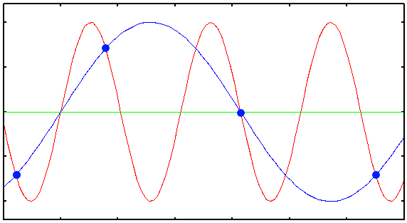 Plot showing the undersampled acquisition of a 1D sinusoidal signal in red. The blue dots are the digital samples taken to attempt to record the red signal. Clearly there are not enough samples taken to reconstruct the original signal. When the blue samples are interpolated, a different periodic structure arises (blue solid line). This effect is called aliasing, and can also occur in microscopy imaging!
Magnification
What determines the microscope PSF, and therefore the resolution and the ideal sampling rate, is not the magnification but mostly the Numerical Aperture. Still, the magnification is relevant to properly map the resolved points onto the detector, specially in the case of a CCD camera. You need a total magnification that correlates the pixel distance in the detector with the ideal sampling distance on the object you are imaging.
For example, in a Wide Field Microscope using a NA = 1.3 objective, Excitation Wavelength 488 nm and Emission Wavelength 520 nm, the ideal sampling rate in the X-Y plane is 100 nm in both directions. If your CCD detector has a lateral pixel size of 6.7 µm (read our FAQ How to calculate the X and Y sample sizes using a CCD camera?) you ideally need a magnification of 6700 / 100 = 67. Higher magnifications lead to oversampling, which is not necessarily bad. Lower magnifications will produce undersampled images which are difficult to process.
Calculations
You can calculate the ideal sampling of your optical conditions using the Nyquist Calculator. NEW: calculate the Nyquist rate with the Nyquist Calculator App. The theory behind it is explained in the Nyquist Rate.
See also Quality Vs Sampling and Bleaching Vs Sampling.