
Table of contents
The Nyquist rate
Basics
It is recommended to read Sampling Density before this article.
The important idea here is that the ideal sampling density during acquisition depends on the optics of the microscope. As the Point Spread Function (PSF) is the basic "brick" of which the images are "built", one should record details at least on the scale of the PSF to gather all the available information. DeConvolution is an operation working on the PSF scale, and the Image Restoration may be useless when the acquisition is done at a larger scale. See Quality Vs Sampling.
Nyquist calculator app and calculator
For a version of our Nyquist app for Android devices, please visit this page. We also offer a free to use Nyquist Calculator online.
Introduction
The Nyquist-Shannon sampling theorem establishes that "when sampling a signal (e.g., converting from an analog signal to digital), the sampling frequency must be greater than twice the Band Width of the input signal in order to be able to reconstruct the original perfectly from the sampled version" (see publications of both Whittaker and Shannon; see reference list below).
The Nyquist criterion determines the minimal Sampling Density needed to capture ALL information from the microscope into the image (see Image Formation). When the sampling distance is larger than the Nyquist distance, information about the image is lost. This UnderSampling condition also gives rise to Aliasing Artifacts. Aliasing artifacts may show up as jagged edges (staircasing) or fringes. These are very hard to remove from the image.
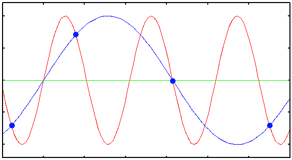 Plot showing the Under Sampled acquisition of a 1D sinusoidal signal. The blue dots are the digital samples taken to record the red signal. Clearly they are not enough to reconstruct the original signal: from them, only the blue wrong signal can be interpolated.
From the point of view of the image information content OverSampling, i.e. sampling at intervals smaller than the Nyquist distance, is harmless except that computation times and storage requirements will be higher. Still, oversampling might lead to longer acquisition times than necessary and therefore to, for example, Bleaching Effects. Often though it is possible to find a compromise between sampling density, line averaging, laser intensity and acquisition time.
Defining the Ideal Sampling in terms of Spatial Resolution is frequently done as a rule of thumb ("sample with half of the Rayleigh Criterion") but this is not exactly correct, and in some cases will lead to UnderSampling (see Pinhole And Bandwidth, for example). The ideal sampling rate is better defined in terms of the system Band Width, which is determined by the Point Spread Function.
Sampling densities
It is very important for the quality of a deconvolution result that all information generated by the optics of the microscope is captured in digital form. It can be shown that if the Sampling Density is higher than a certain value all information about the object is captured. We will call this value the Critical Sampling Distance, corresponding to the Nyquist rate. Apart from practical problems like bleaching, acquisition time and data size there is no objection at all against using a smaller sampling distance than the critical distance (OverSampling), to the contrary.
The following figure shows the dependency of this critical sampling distance on the objective Numerical Aperture (NA) for specific WaveLengths. To apply these curves to different wavelength you can simply scale the vertical axis with the wavelength. Example: you are working with a Wide Field Microscope (WF) with NA 1.3 at Emission Wavelength 570 nm. From the plot you read that the critical lateral Nyquist sampling distance at 500 nm emission is 95 nm, so in your case this becomes 570/500 × 95 nm = 108 nm.
Critical sampling distance vs. NA. The curves above show the Critical Sampling Distance in axial and lateral directions for wide-field and confocal microscopes. The emission wavelength in both cases is 500 nm.
In the confocal case it is the excitation wavelength which determines the Nyquist sample distance. In theory the Pinhole Radius plays no role, but larger pinholes strongly attenuate fine structures at the resolution limit. Therefore, as a rule of thumb, with a common pinhole diameter of 1 Airy disk the lateral critical sampling distance may be increased by 50% with negligible loss of information. In cases were the pinhole is much larger, the lateral imaging properties much resemble those of a WF system and the sampling distance can be set accordingly. We do not recommend to increase the axial sampling distance appreciably beyond the critical distance.
Calculator
|
| You can use the Nyquist Calculator to find which ideal sampling density you should use to acquire your images, depending on the optical conditions. |
Equations
The above plot is just meant as orientation for the axial sampling, as despite the varying NA it assumes a fixed Refractive Index of 1.51. The detailed equations used to make that plot follow.
Widefield case
The Nyquist critical sampling distance for a conventional fluorescence Wide Field Microscope is given by:
$$\Delta_x=\frac{\lambda_{em}}{4 n \sin(\alpha)}$$ $$\Delta_z=\frac{\lambda_{em}}{2 n (1-\cos(\alpha))}$$ (EQ 1)
with n the Lens Refractive Index (usually 1.515 for immersion oil), α the half-aperture angle of the objective, λem the Emission Wavelength, and Δx, Δz the Sampling Distances in the lateral and axial direction respectively. This is about one half of the microscope resolution. (Note that the sampling for a widefield microscope does not rely on the excitation wavelength.)
In the equation above α can be computed from
$$\alpha=\arcsin(\text{NA}/n)$$ (EQ 2)
with NA the Numerical Aperture. From (EQ 2) we find the relation between the numerical aperture and the Lens Refractive Index.
$$\text{NA}=n\sin(\alpha)$$ (EQ 3)
We see now that NA is always smaller than n since sin(α) is always smaller than one.
If you set in your parameter list the NA to 1.2 and the refractive index to 1.2 or less, the Huygens Software will display "Warning: total reflection at glass/medium interface, setting G_alpha to pi/2", while trying to generate a Theoretical Psf.
For a 1.3 N.A. oil immersion objective α is about 1.0 radian, close to 60 degrees.
Nyquist rate and bandwidth
The Δx and Δz values discussed above are distances, corresponding with half the cycle length of the highest spatial frequency passed by the system. The Nyquist rate (cycles per unit distance) is therefore
$$F_{\text{Nyquist},x}=\frac{1}{2\Delta_x}$$ and $$F_{\text{Nyquist},z}=\frac{1}{2\Delta_z}$$
This is often referred to as the system Band Width.
Confocal case
For a Confocal Microscope the above mentioned sampling distances for a conventional widefield microscope must be divided by 2!!!.
For a confocal, the total Point Spread Function (PSF) is the product of the independent excitation and detection point spread functions. Since the wavelength for excitation and emission are approximately equal - and the blurring effect of a finite sized detection pinhole doesn't alter the bandwidth of the detection system, the Band Width of the overall PSF is twice as large. Because of this doubling of the system bandwidth the confocal Nyquist sampling distance is half of the equivalent widefield sampling distance.
$$\Delta_x=\frac{\lambda_{ex}}{8 n \sin(\alpha)}$$ $$\Delta_z=\frac{\lambda_{ex}}{4 n (1-\cos(\alpha))}$$ (EQ 4)
To compute the confocal sampling distance, the Excitation Wavelength λex should be used.
Doubling the bandwidth does not imply that the resolution is doubled, at least not using the Rayleigh Criterion for resolution. Actually, with this criterion lateral resolution is only improved in a factor of about 1.4. The doubling of the bandwidth is also reflected, in spatial terms, in the improvement of the contrast.
Although the confocal microscope is able to transmit twice as fine details as the widefield microscope, unfortunately it attenuates these very strongly. Beyond say 60% of the highest frequency practically nothing is transmitted, especially for not-ideal pinhole cases. Therefore, if you use the theoretical Nyquist sampling rate you are very much in the clear. But it is defensible to use a practical Nyquist rate at 60% of the theoretical rate, (about one sample per 50 / 0.6 = 80 nm).
In the widefield case high spatial frequencies are also attenuated as the limit is approached, but to a much lesser degree than in the confocal case. Therefore we recommend not to undersample widefield images.
Multi-photon case
In the case of a Multi Photon Microscope with k-photon excitation, the excitation point spread function is raised to the k-th power, and therefore the theoretical Band Width is multiplied by k. But this is compensated by the enlargement of the Excitation Wavelength, that compared to the single photon case is also multiplied by approximately k. And the limits of the bandwidth are very attenuated.
As a result, an appropriate sampling rate in the case of large or no pinhole (please read our info page How to treat 2-photon data in Huygens) comes from using the same equations as in the widefield case above, with the actual Excitation Wavelength divided by the Photon Count k:
$$\Delta_x=\frac{\lambda_{ex}}{4 k n \sin(\alpha)}$$ $$\Delta_z=\frac{\lambda_{ex}}{2 k n (1-\cos(\alpha))}$$ (EQ 5)
Importantly, the 3D shape of the band-pass volume is very different: while the widefield area has a wedge at the center causing the large widefield blur cones, the multi-photon bandpass volume has no such defects.
A typical example
A typical confocal microscope with excitation in the 480-520 nm range, and a 1.3 NA objective should therefore be sampled with a lateral sampling distance of 50nm and an axial sampling distance of 150nm. Experienced confocal microscope operators might object that such small sampling distances will give rise to Bleaching Effects. This is true when one aims to achieve an apparent Signal To Noise Ratio which is the same as in more coarsely sampled images. However, the restoration procedure will improve the apparent Signal/Noise ratio dramatically!!! Therefore, densely sampled images can be of lower Signal/Noise than usual. In effect one may exchange averaging count for Sampling Distance. For example when four times more samples are taken from the same volume in the specimen, the averaging count can be reduced by the same factor.
Suggestions for further reading
See the section on image sampling and quantization (section 2.3) in `Digital Image Processing' by Gonzalez & Woods (ISBN 0201180758) for details on this topic.
See the FAQ for the answer on the following questions:
- What is the maximal voxel size at which Huygens can still do a good job?
- The better sampled the PSF, the better the deconvolution result?.
Search the FAQ for "Nyquist".
References for the equations used on this page are:
- Wilson, T. and Tan J.B. Three dimensional image reconstruction in conventional and confocal microscopy. (1993) BioImaging 1:176-184.
- Sheppard, C.J.R., A. Choudhury and J. Gannaway. Electromagnetic field near the focus of wide-angular lens and mirror systems. IEE J. (1977) Microwaves, Opt. Acoust. 1, 129-132.
- Sheppard, C.J.R. The spatial frequency cut-off in three-dimensional imaging. (1986a). Optik 72 No. 4 131-133.
- Sheppard, C.J.R.The spatial frequency cut-off in three-dimensional imaging II. (1986b). Optik 74 No. 3, pp. 128-129.
References regarding the sampling theorem are:
- Whittaker E.T., On the functions which are represented by expansions of the interpolation theory (1915). Proc. Roy. Soc. Edinburgh Sect. A, 25:181.
- Shannon C.E., Communications in the presence of noise. (1949) Proc. IRE, 37:10
- Goodman J.W. Introduction to fourier optics 2nd ed. (1986) McGraw-Hill Book Companies Inc.
Links: