Huygens Deconvolution: Restore microscopy images

"The job of image restoration is to figure out what the instrument is actually trying to tell you''. -- Prof. E.R. Pike, King's College, London.

Introduction

Deconvolution is a mathematical operation used in Image Restoration to recover an image that is degraded by a physical process which can be described by the opposite operation, a convolution. This is the case in image formation by optical systems as used in microscopy and astronomy, but also in seismic measurements.

In microscopy this convolution process mathematically explains the formation of an image that is degraded by blurring and noise. The blurring is largely due to diffraction limited imaging by the instrument. The noise is usually photon noise, a term that refers to the inherent natural variation of the incident photon flux.

The degree of spreading (blurring) of a single pointlike (Sub Resolution) object is a measure for the quality of an optical system. The 3D blurry image of such a single point light source is usually called the Point Spread Function (PSF).

Image formation

PSFs play an important role in the image formation theory of the fluorescent microscope. The reason for this is that in incoherent imaging systems such as fluorescent microscopes the image formation process is linear and described by Linear System theory. This means that when two objects A and B are imaged simultaneously, the result is equal to the sum of the independently imaged objects. In other words: the imaging of A is unaffected by the imaging of B and vice versa.

As a result of the linearity property the image of any object can be computed by chopping up the object in parts, image each of these, and subsequently sum the results. When one chops up the object in extremely small parts, i.e. point objects of varying height, the image is computed as a sum of PSFs, each shifted to the location and scaled according to the intensity of the corresponding point. In conclusion: the imaging in the fluorescent microscope is completely described by its PSF.

For more details read Image Formation.

Convolution

You can imagine that the image is formed in your microscope by replacing every original Sub Resolution light source by its 3D PSF (multiplied by the correspondent intensity). Looking only at one XZ slice of the 3D image, the result is formed like this:

(Fig. 1)

This process is mathematically described by a convolution equation of the form

$$ g\ =\ f\, \ast\, h $$ (Eq. 1)

where the image g arises from the convolution of the real light sources f (the object) and the PSF h. The convolution operator * implies an integral all over the space:

$$ g = f \ast h = \int\limits_{-\infty}^{\infty}\int\limits_{-\infty}^{\infty}\int\limits_{-\infty}^{\infty} f(\vec{x}') h(\vec{x} - \vec{x}')\ d^3\vec{x}' $$ (Eq. 2)

Interpretation

You can interpret equation 2 as follows: the recorded intensity in a VoXel located at $$ \vec x = (x,\, y,\, z) $$ of the image \( g (\vec x) \) arises from the contributions of all points of the object f, their real intensities weighted by the PSF h depending on the distance to the considered point.

Calculation

That means that for each VoXel located at $$ \vec x = (x,\, y,\, z) $$ the overlap between the object function f and the (shifted) PSF h must be calculated. Computing this overlap involves computing and summing the value of \( f(\vec x)\ h(\vec x - \vec x') \) in the entire image. Having N voxels in the whole image, the computational cost is of the order of N².

But this can be improved. An important theorem of Fourier theory, the convolution theorem, states that the Fourier Transforms G, F H of g, f, h respectively are related by simply a multiplication:

$$ G = F \cdot H $$. (Eq. 3)

This means that a convolution can be computed by the following steps:

1. Compute the Fourier transforms F and H of f and h
2. Multiply F times H to obtain G
3. Transform G back to g, the convolved image.

Because Fourier transforms require a number of operations in the order of N log(N), this is more efficient than the previous integral.

To see how the application of different PSF's affect the imaging of an object, read the Cookie Cutter.

Deconvolution

If convolution implies replacing every original (sub-resolution) light source by its correspondent PSF to produce a blurry image, the restoration procedure would go the opposite way, collecting all this spread light and putting it back to its original location. That would produce a better representation of the real object, clearer to our eyes. (This increases the Dynamic Range of the image, and causes the background regions to look darker!!!).

Mathematically speaking, deconvolution is just solving the abovementioned Eq. 1, where you know the convolved image g and the PSF h, to obtain the original light distribution f: an representation of the "real" object.

The relation in Eq. 3 would seem to imply that it is possible to obtain the object function F by Inverse Filtering, just by dividing F = G/H. But due to the bandlimited character of H it has zeros outside a certain region (see Cookie Cutter), resulting in a division by zero for many spatial frequencies. Also, in a real general case the Photon Noise must be taken into account, so the equation that we actually have to solve is not Eq. 1, but this:

$$ k\ =\ f\, \ast\, h\ +\ \epsilon $$ (Eq. 4)

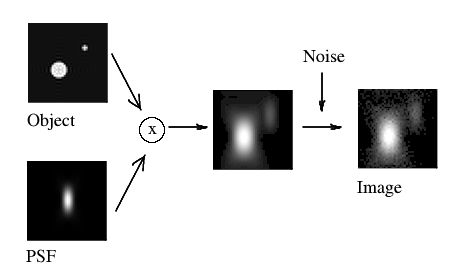(Fig. 2)

where the acquired image k arises from the convolution of the real light sources f and the PSF h, plus the photon noise ε. The division of ε by H would lead to extreme noise amplification and therefore tremendous artifacts due to the large areas of small values of H within the passband. (Also, we can not simply substract ε from k, as we can not know what is the exact noise distribution).

Thus, inverse filtering will never allow us to recover the true object function f. Instead, we must try to find an estimate f' which satisfies a sensible criterion, and is stable in the presence of noise.

Some deconvolution methods (like Blind Deconvolution) try to solve equation 4 without knowing the PSF term h. Although some constraints can be applied, this is always risky, as it introduces a lot of indetermination in the solution of the equation. (How many solutions x, y can you find for an algebraical equation of the form x × y = 5?) These methods are also currently lacking of any scientific validation when applied to microscopy.

We must go for another solution.

The way Huygens Deconvolution Software works

The Huygens Software of Scientific Volume Imaging enables you to obtain a PSF in two ways:

• automatically computing a Theoretical Psf based on known Microscopic Parameters and a model of the microscope, or
• distilling an Experimental Psf from spherical bead images, after Recording Beads.

In the second case, given a model of the bead shape, the PSF is computed 'distilled' which its convolution with the bead model matches the measured bead image. That can be understood looking back at figure 1 and equation 1. Now we know how the object f is (the exact size of the spherical bead must be known) and we have acquired its image g, thus we can distill the remaining unknown term h in the equation.

Once a PSF is provided Huygens can use different mathematical algorithms to effectively solve the convolution equation 4 and do deconvolution:

• Classic Maximum Likelihood Estimation
• Quick Maximum Likelihood Estimation
• Iterative Constrained Tikhonov-Miller
• Quick Tikhonov-Miller
• Good's Roughness Maximum Likelihood Estimation

The Classic Maximum Likelihood Estimation (CMLE) is the most general Restoration Method available, valid for almost any kind of images. It is based on the idea of iteratively optimizing the likelihood of an estimate of the object given the measured image and the PSF. The object estimate is in the form of a regular 3D image. The likelihood in this procedure is computed by a Quality Criterion under the assumption that the Photon Noise is governed by Poisson statistics. (Photoelectrons collected by a detector exhibit a Poisson Distribution and have a square root relationship between signal and noise). For this reason it is optimally suited for low-signal images. In addition, it is well suited for restoring images of point- line- or plane like objects. See Maximum Likelihood Estimation for more details.

There are however situations in which other algorithms come to front, for example when deconvolving 3D-time series, which is very compute-intensive. In this case you may consider to use Quick Maximum Likelihood Estimation-time (QMLE) which is much faster than the CMLE-time and will give excellent results as well. With the Good's roughness Maximum Likelihood Estimation algorithm (GLME) you will see improved handling of very noisy images, in especially STED and confocal data.

An advantage of using measured PSF as in Huygens is that in essence it requires you to calibrate your microscope, and stimulates the use of standard protocols for imaging. Together, these will ensure correct functioning of the microscope and vastly increase the quality and reliability of the microscopic data itself, and with that of the deconvolution results.

Lastly, an advantage of theoretical or measured PSFs is that they facilitate construction of very fast algorithms like the QMLE present in Huygens Essential and Professional, and in the Workflow Processor. Iterations in QMLE are about five times more effective than CMLE iterations and require less time per iteration.

Images affected by Spherical Aberration due to a Refractive Index Mismatch are better restored with Huygens Software through the use of depth-dependent PSF's (see Parameter Variation).

Huygens algorithms generally do Intensity Preservation.

See the Huygens restoration applied to some accessible images in Convolving Trains.

Validation

The CMLE method used in Huygens is backed up by quite some scientific literature. We mention here just three relevant examples (follow the previous link for a longer list):

• Verschure P.J., van der Kraan I., Manders E.M.M. and van Driel R. Spatial relationship between transcription sites and chromosome territories. J. Cell Biology (1999) 147, 1, pp 13-24 (get pdf).
• Visser A.E. and Aten J.A. Chromosomes as well as chromosomal subdomains constitute distinct units in interphase nuclei. J. Cell Science (1999) 112, pp 3353-3360 (get pdf).
• Hell S.W., Schrader M. and Van Der Voort H.T.M. Far-Field fluorescence microscopy with three-dimensional resolution in the 100-nm Range. J. of Microscopy (1997) 187 Pt1, pp 1-7 (get pdf).

Examples

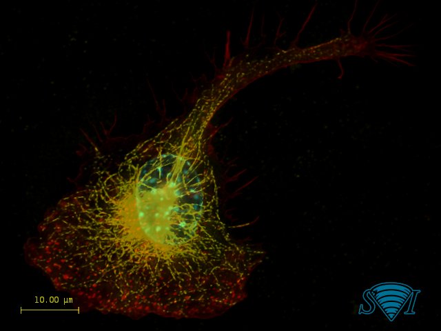
Experimental point spread functions were generated for the red, green, and blue channels on an epifluorescence microscope and then used to deconvolve a standard Invitrogen Floucells #1 prepared slide, containing bovine pulmonary artery endothelial cells stained for mitochondria (red), F-actin (green), and nuclei (blue). Before (left) and after (right) deconvolution images were merged side by side to display the power of deconvolution. Image created by Dr. Jeff Tucker and Dr. Holly Rutledge from NIEHS, NIH, USA

Macrophage fluorescently stained for tubulin (yellow/green), actin (red) and the nucleus (DAPI, blue). This images is a MIP of the deconvolved data and if you mouse over it you will see the raw data. Image recorded with a Wide Field Microscope by Dr. James Evans, Whitehead Institute, MIT Boston MA, USA.

More information

See Doing Deconvolution for special topics and references.

Testing Huygens Deconvolution

You can download the Huygens software from our website for free. After installing and starting the Huygens software, you can request a temporary test license to explore the Huygens deconvolution, visualization and restoration options. Feel free to try out all our products for free. There are also many FreeWare tools in the software that can run without any license.

References

Click here for more references.

References

AII amacrine cells: quantitative reconstruction and morphometric analysis of electrophysiologically identified cells in live rat retinal slices imaged with multi-photon excitation microscopy. Brains Structure & Function 1–32 (2016) This paper describes in much detail the optimal imaging and deconvolutution settings that were applied.
Correlated confocal and super-resolution imaging by VividSTORM. Nature Protocols 11, 163–183 (2016) Huygens deconvolution was used to create the cover of this issue of Nature Protocols.
Viruses 2018, 10(1), 28; doi:10.3390/v10010028 Huygens was used for deconvolution.